Description
Using data from Taarifa and the Tanzanian Ministry of Water, I predict which pumps are functional, which need some repairs, and which don't work at all. This is an intermediate-level practice competition on DrivenData. I predict one of these three classes based on a number of variables about what kind of pump is operating, when it was installed, and how it is managed using Random Forest.
The data for this comeptition comes from the Taarifa waterpoints dashboard, which aggregates data from the Tanzania Ministry of Water.
In their own words:
Taarifa is an open source platform for the crowd sourced reporting and triaging of infrastructure related issues. Think of it as a bug tracker for the real world which helps to engage citizens with their local government. We are currently working on an Innovation Project in Tanzania, with various partners. (More about Taarifa can be found HERE)
This will be a high level walk-through of my submission.
Imports & Admin
First of all, lets get the admin out of the way. These are the packages I will be using throughout the analysis. These are also the references to the raw data that I will be reading the data into. Note that the only model I will be using is the random forest model and the reasoning behind this is later explained. After creating dummy variables for the my output variables, I then concatenate the resulting dataframe to my training data frame so I can work on cleaning the data together, being aware of information leakage in my feature engineering process.
Data Info
Here we can see that the test set is 4 times smaller than the training dataset. This should be fine as we know the test set is a taken from the same source as the training data. Then following this, we can assess how many unique values are within each of the columns then we can go from there. First order of business is assessing null values and whether we want to keep them and replace their values or drop them completely.
Boolean to Binary
I then begin to build functions that I can nest within a bigger function that clean up specific areas of the dataset. For example, from the previous code cell, showing the number of unique values within each feature column, showed a few categories with 3 unique values. After further investigation, it was clear these values were "True", "False" and "NaN" (Not a Number). To maintain simplicity, I replaced the NaN values with "False" then assigned 1 to True and 0 to False, so that the models I train on this data are able to use this data.
Level Combination
The unique feature counter shows that the funder and installer had a rather high number of categories. So, I decided to break these down into 10 groups based on their frequency. The above code block shows functions that break down the respective frequencies into groups and returns the values category. Another function uses the previous in order to clean up the dataset as shown. I use the same method for combining levels with the installer feature which had a high number of categories.
Response Rate Level Combination
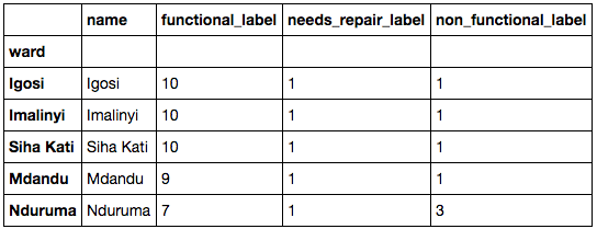
.Here I use a similar method for a number of other variables with a high number of categories, however, I utilise the response rate for each of the unique values and their levels. The first function above is a truncated view of the full function that categorises each entry based on their score. The next set of functions are used to calculate the response rate for each of the different categories.
The rest of the code block is assigned to organising each of these "ward" values with a category in each output variable option based on their response rates in their respective output options. This is then stored in a dictionary for each option so that it can be used in both the larger cleaning function for both the training and test data sets. I've used the same method for a number of other appropriate features that have been identified in the unique value count earlier.
The rest of the code block is assigned to organising each of these "ward" values with a category in each output variable option based on their response rates in their respective output options. This is then stored in a dictionary for each option so that it can be used in both the larger cleaning function for both the training and test data sets. I've used the same method for a number of other appropriate features that have been identified in the unique value count earlier.
Feature Dropping
Here I drop a number of redundant features. I label these fields as redundant as they do not provide any additional information. There are similar features for each of these that are used instead and are labeled into categories so that the models can handle the variables.
Feature Cleaning & Engineering
Here I create a feature that indicates how many years the pump has been around since construction to the date the record was recorded. I then assign categories to each of the features labelled above. These are built into a larger cleaning function so that the same transformations can be applied to the test dataset prior to making the predictions.
Feature Transformation
Having looked at the distribution of each of the variables, I decided to transform a few continuous variables using a lambda x: np.log(x+1) function. This transforms 0 values to 0 which is also quite handy.
Random Forest Modelling
Our dataset that we are going to predict from is full of both, continuous, binary and categorical features, therefore, with this knowledge, it would make sense to use a random forest model seeing as this ensemble method is able to cater for these feature types. a quick run of this model yields a 99.75% accuracy based on all the training set data. It is quite likely that this is overfitting and so a cross validation is performed in order to get a better idea as to how well the model is performing.
Using a K=10 K-fold cross validation we are able to subset the data and build and run 10 different random forest models and test them on out of sample data to get a better indication as to how they perform. following the cross validation, we can see hat averaging across 10 models, the Random Forest model performed with an accuracy of 80.81% ranging from 79.93% to 81.82%.
Here i then repeat the process of building, testing and predicting the values using 200 iterations. This is to account for the random element within the model choice. By repeating the process a large number of times, we get a more reliable rounded view of how the model is performing and we are able to use more reliable results in our predictions. The Random Forest Algorithm, as the name suggests, has an element of randomness built in that results in two models not necessarily producing the same output. We can see this phenomenon in the differences in accuracies in our precious cross validation.
Submission
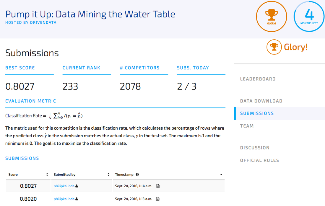
This is the bit of code just to create the submission to post. I managed to come 233 out of 2078, which isn't too bad. I'll be looking into how I could improve this model at a later stage once I discover new algorithms and feature handling techniques. These are constantly being developed every day! One of the great things about Data Science! An extremely dynamic field!