Background
Hackerrank is a platform where fellow coders come together to learn more about coding, compete against each other and showcase their skills. There are a number of challenges and tutorials that are either specific to a topic like algorithms, Machine Learning or Security or to a programming language like C++, Java or Python. They often host a number of competitions in these fields or languages. This gives fellow coders to compete against their piers in the hopes to earn badges and reputation within the community as a great coder or specialist in your field. Here, I will be briefly walking you through my submission to one of the challenges presented in the Machine Learning competition.
Description
In this challenge, we are presented with a dataset that details information regarding users of the hackerrank site and emails sent to these users. The objective of the challenge is to predict whether or not a user will open the email or not. We are given a training set that we are to use to build the model and a test set against which we will predict in order to produce our submission.
Admin & Imports
Here are all the imports that I used to build my submission. If you are familiar with some of these imports, this should give you an idea as to how I look to approach the problem and the models that I used to get to my submission. Just to run through quickly. Pandas is what I'll be using for storing data into dataframes as the data is not purely numeric, otherwise I would would be more inclined to use just numpy and matrix multiplication as this is computationally faster. I use numpy here for numerical calculations throughout.I use matplotlib in order to plot graphs to visualise the data. I use time and datetime to parse dates and extract features from the dates. I use a number of imports form sklearn for the modelling process. This includes cross validation of models as well as building the actual models. I use xgboost as a separate model also to provide a wide range of models in order to assess which could be a better choice. If I decide to go with just one model. The settings are just for me to block specific caveats that I am aware of and to display all the columns as I scroll through. I prefer to look through the whole dataset.
The Data
Here we can read the data in and have a quick look at the data's dimensions, both the training dataset and the test set. This shows us that there are 486,048 records in the training dataset and 207,424 records in the test dataset that we will be predicting against in our final submission. Moving onto how I have coded and go about manipulating the dataset, may I just highlight that I have taken advantage of the computational efficiency and ease of structure of functional programming. OK, Let's start off by looking at the training dataset.
Looking at the data, we will need to create some numeric fields in order for us to use some of the models we want in order to predict our dependant variables. A lot of fields have boolean values in order to determine the presence of a certain variable within the training set. to use these in our model we can convert these into binary outputs to represent the respective boolean value ie. True -> 1; False -> 0.
Data Handling & Feature Extraction
We have a number of date fields from which we can extract features. Lets have a look at some of these.
My thought processes were:
1. Perhaps if an email is sent on a weekend or a weekday, this could potentially influence the probability of the user opening the email. Here I use the same numeric representation of 1 for if the email is sent on a weekend and 0 if it wasn't.
2. I wonder if the month in which it was sent would have any affect on being open? Perhaps, they would be less likely to be opened during summer because they're too busy on a beach enjoying the sun somewhere hot, disconnected from the net. Here I parse the dates and created a categorical variable with 12 categories.
3. I wonder if the time of day in which it was sent had an effect? From this query, 24 categories were created in order to represent each hour of the day.
4. I wonder if the time between when the hacker was last online and the email was sent can be a predictive variable in assessing whether or not the user opens the email. Maybe the user is less likely if they are already engaged with the platform? So here, the dates are parsed and subtracted from each other and added to the DataFrame.
5. I wonder if the time between when the hacker first created their profile and the email sent can also be a significant predictor in determining whether or not the user opens the email. So here, the dates are parsed and subtracted from each other and added to the DataFrame, just as the previous variable.
Days between last online and email sent
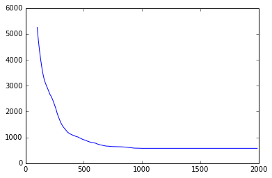
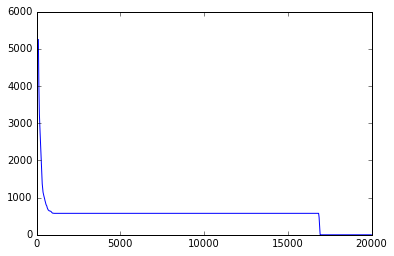
Looking at the days since online and day the email was sent, we get some pretty extreme outliers. Here we have a look at the length of the list relative to the number of days between the hackers last online status and the date the email was sent. This plateaus at 1,000 and then dips down to 0 16,000 points later. Starting from 1000, there isn’t that many items in the list so I decided to cut off the data at that point and state that those greater than 1000, I will treat as 1000. I could alternatively take the log(x+1) of the variable and reduce the variation in the variable but I chose this approach for testing out so far and keep as much variability in the variable as possible before normalising.
Normalising
There are a number of variables that contain counts of specific metrics, however these are cumulative. What I was hoping to do is normalise this so that I can generalise the variables. What I have done is obtained values for ranges and subsequently removed the cumulative nature of the variables and I have divided each of these discrete counts by their totals in order to get a proportion. This allows for hackers of all lifespans to be compared to evenly. I have already captured a variable to detail the age of the hackers account through the previous feature extraction method around the dates. if there are cases where there are no counts whatsoever, anything divided by 0, even 0, return a NaN (Not a Number) object. To deal with this, I add a line to fill in the areas of the variable that are NaN with 0 instead.
Following the production of all these functions, we need to apply them to the relevant columns in the data in order to produce a cleaned dataset which we can run through our models. This clean_data() function is used as a means to run the functions above and select the appropriate columns to carry forward into the returned data frame. Within this function you can pass in whether you are cleaning the training dataset, which would return the target column as well as the independent variables used to train the model that have been cleaned, or the test dataset, which wouldn’t contain the target column, but all the other relevant columns used to model. The final elememnts of the function concatenate all the relevant columns and removes any NaN values and replaces them with 0 as to patch the returned values of 0 / 0 = NaN.
Models
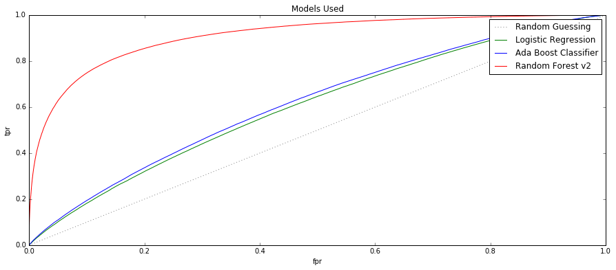
Now that we have our training and test data, let’s have a look at the models that we can use and have a look as to which of them can produce the best predictions. I had a look at the Logistic Regression which yielded the result of 66. 9734% accuracy. I had a look at Support Vector Machines which was marginally worse with 66.9306% accuracy. I also had a look at an AdaBoostClassifier which had an improved score of 67.1835% and I also had a look at random forest which was much better with a score of 78.9836% accuracy. I then also had a look at the ROC score in order to visualise the difference in performance of these models and the random forest showed to be a much better model to the other models.
Models Used - ROC Curves
These ROC Curves make it pretty obvious that the random forest out-performed the rest of the models. This shows that the random forest was more likely to rank a random positive observation higher than a random negative observation.
That’s great, we can finish with that, but I thought that perhaps we can optimise our models and even use an ensemble of models in order to increase our accuracy and robustness of the model. After running a Grid search, I was able to find optimal parameters and have applied them to the ensemble of models. Back to my functional programming approach, I made a function that takes the training dataset, the test dataset, a sample size and a threshold.
These parameters enable you to tweak the model to achieve optimal results relevant to your specifications. The sample size is a percentage of the training set that you wish to train the model. These are based on a stratified approach to ensure that the data used in training reflect the true dataset as much as possible. The threshold is the point at which each of the models predict the probability of being in one class over another. This can be set dependent on your business requirements. The ensemble of models resulted in an accuracy score of 81.3675% making it the best model to use.
These parameters enable you to tweak the model to achieve optimal results relevant to your specifications. The sample size is a percentage of the training set that you wish to train the model. These are based on a stratified approach to ensure that the data used in training reflect the true dataset as much as possible. The threshold is the point at which each of the models predict the probability of being in one class over another. This can be set dependent on your business requirements. The ensemble of models resulted in an accuracy score of 81.3675% making it the best model to use.
Improvements
If there was more time, throughout the competition, I would have looked to grid search a wider range of parameters. I would also liked to have explored identifying patterns and structures in terms of groups using Unsupervised methods and relating those structures to the test set via a mapping exercise. I could have tried a number of different models with different treatments of variables. I could have utilised a more scientific approach to setting the thresholds. There are a number of different things I could have done and would have, if it were my full time job, however, in the interest of time the model built was sufficient.


